Market Mindset

The FX Carry Trade: CHF/COP & USD/TRY
What is the FX Carry Trade?

A carry trade is a trading strategy at the core of active currency management. It sees an investor borrow capital in a currency that has a low interest environment, such as Japan (0.75%), and invest the borrowed funds into a currency where there is a high interest rate, such as Mexico, Brazil, and Egypt (7%, 15%, and 20% relatively). These latter target currencies offer a higher yield, and this can be denoted as a ‘risk-on environment’. This strategy intends to gain profit from the ex-ante positive interest rate differential.

This strategy, by logic, seems an effortless and remunerative route to achieve simple profit. In reality, this carry trade faces more predicaments, one of which is the theory onUncovered Interest Rate Parity (UIP). Since anFX carry trade is usually conducted using forwards (although futures and swaps can also be used). The UIP theory states that this carry profit is harder to achieve because when forward products are used, the forward exchange rate is meant to be higher to reflect the spot rate, and close out this interest rate differential gap. If UIP theory holds up the expected return should end up being zero.

Nonetheless, the FX carry trade is still postulated here as a possible strategy, due to the frequent failure of UIP to materialise, which is coined the ‘carry trade puzzle’. This is where currencies with high interest rates, tend to appreciate more – going against UIP, (which proposes these currencies should theoretically depreciate). Thus, the subsequent buying pressure on the quote currency enables it to appreciate even more, this enables the trade to be existentially embedded.

An article from 2014, by Daneil, Hodrick and Lu, advances that the time-varying dollar exposure of the carry trade is at the core of the carry trade puzzle. The US dollar matters to carry trades, even when both the base currency and quote currency are not USD. Carry trades are not just bilateral transactions; they are relative, and load on a global risk factor – the US dollar.
Yet, this sensitivity is not constant, the beta of the carry returns changes over time. When a carry trade expects high returns in a risk-on environment the dollar exposure can seem small or negative. In the parallel situation, in a risk-off environment, the dollar strengthens, investors unwind carry positions, and dollar exposure will then grow and be positive, which is when returns will be the worst for carry trade positions. This can help explain why the carry trade puzzle occurs. In essence, UIP theory accounts for constant risk and does not encompass the dollar’s tie to non-dollar carry trades, and that the dollar’s risk is nonlinear.

Going beyond this, high interest rate currencies, for example the Turkish lira and Egyptian pound, tend to trade at forward discounts (a currencies forward rate is lower than its spot rate), relative to the low interest rates currencies. In comparison to low interest rate currencies, which trade at forward discounts (the currencies forward rate is higher than its spot rate). Accordingly, the carry trade still suffices by carrying out a long position in forward markets where forward discounts are present. On the parallel side, the carry trade can still be implemented when going short in currencies where a forward premium is present.

Additionally, this trading strategy comes with another significant risk. Countries with a high interest rate, are usually positioned against highly volatile markets tied to a fickle geopolitical landscape. Unwinding of risky positions can happen when volatility takes form. As such, carry trades work best in quiet markets.

The discussion on the risk premium on a FX carry trade is further nuanced than this and can be divulged more by looking at market variance. Market variance in FX, involves measuring how much an exchange rate deviates from the average mean trend over a time period. Higher variance measure means there are larger, jumpier, and more unpredictable moves from the average. A low variance measure, indicates smaller, steadier and more predictable moves from the average. Market variance is the average of the squared deviations from the mean return. On a futile level, market variance is the sum of average variance + average correlation. Average variance can be broken down into how volatile, currencies are on average, while the average correlation shows much currencies move together.

A research article from Cenedese, Sarno, and Tsiakas (2014) explores on how market variance has a predictive power for indicating carry trade returns. This quoted ‘predictive power’, is primarily dependent on average variance, which also has a noticeable negative effect on the left tail of future carry trade returns. Moreover, the trustworthiness of market variance as a predictability tool of carry trade returns is shown to be more reliable in crucial periods.

FX Carry Trade Suggestions: CHF/COP and USD/TRY

CHF/COP
- Swiss Rate Hold
Many central banks in 2026 are seeing this year as an end to their rate-cutting cycle, evident by The Fed’s rate hold on January 28^th, followed by previous cuts in 2025. The Swiss National Bank has the same sentiment of holding rates for the foreseeable future into 2026 at 0%, effective since June 2025. The Swiss central bank, appears to have no desire to increase rates, due to their low inflation, hovering year-on-year at around 0.0% to 0.1%, which is well below their aim. Therefore, CHF serves as an ample base currency here.
- The Dollar Connection
As uncovered previously, the dollar is tied to a carry trade even if not it is not involved. CHF is a safe-haven currency similar to USD, and due to a weakening dollar, other alike safe-haven currencies see demand fall. This creates an advantageous ‘risk-on’ environment, capital is encouraged to flow into high-yield currencies, in search for yield elsewhere, which puts a CHF/COP carry trade in good standing. If the dollar were to see a reversal and begin to strengthen, this could be a potential risk, as capital could be diverted into safer currencies once more.
- Colombia’s Monetary Policy
News coming out on January Friday 30^th, reports how Columbia’s central bank has raised its base rate to 10.25%. This is an impactful contractionary policy movement, as this 100bp rise, is the first-rate hike in the past 3 years. This comes out following the report that core inflation of the nation picked up in December 2025 to 5.1%, with their aim of 3%. This attempt to inhibit prices, comes after an increase of 23.7% to the country’s minimum wage by Colombia’s president in December 2025.

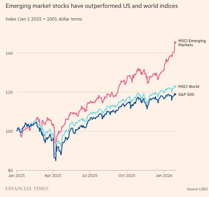
EM currencies have, according to the FT ‘made a roaring start’ in 2026, with Turkey, Brazil, Chile, Mexico, and others gaining 10% in dollar terms in January of this year. Colombia and Korea have performed the best with 20% gain in dollar terms. This is in part due to the weakening dollar, and also surged on with EM stocks outperforming other indices respectively, the US with the S&P 500, and the MSCI World seen below.

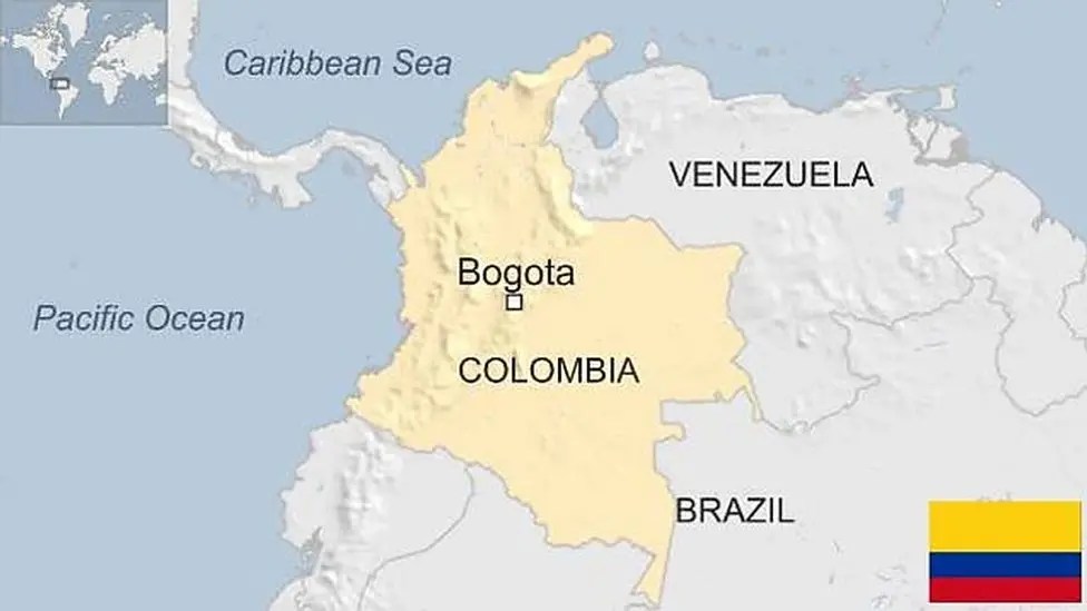
The risk premium on CHF/COP, is the geopolitical state of Colombia. This is in lieu of the backdrop of Venezuela and their tumultuous economic and political proceedings since January. Colombia has a forthcoming presidential election in May 2026; polls are unclear what the projections are, this will have to be watched closely in the run up to May. There is some positive outlook for Colombia, following the optimistic meeting between President Gustavo and President Trump on 3^rd February, with the talk between the two deemed ‘constructive’. Their tricky relationship over the past year has been one damped by tensions around drug-trafficking in the Latin American nation, in which Trump denounced Gustavo was not doing enough, even turning a blind eye to the miss happenings. This positive feedback provides some assurance to investors regarding the stability of COP moving forward into 2026, despite an imminent election.

USD/TRY

For this second exotic currency pair suggestion – one with a somewhat lower risk premium is proposed. USD/TRY is an ample suggestion and a common FX carry trade, and more predictable than CHF/COP. USD is better served as the base currency over CHF in this instance, as USD/TRY is a much more liquid pair, and has lower transaction costs and faster execution, as CHF/TRY is traded much less.

As aforementioned, the Fed is contestably seeing the end of their rate-cutting cycle, after their most recent hold. Rates are forecasted to remain steady by JPMorgan this year between 3.5% to 3.75%, with one singular rate expected for 2026. On top of this, the value of the dollar as widely known, has fallen drastically in 2025, with the dollar index dropping nearly 10-11% by the year end of 2025. Last week, Tuesday 27^th saw the dollar hit a four-year low. The weakness of the dollar is still expected to sustain, but at a less exponential rate as observed in 2025. Accordingly, the dollar seems a sufficient choice for a base currency in a carry trade.
- Turkish Monetary Policy
Turkey is also entering into a rate-cutting cycle, and has now cut 100bps from 38% in December 2025, to 37% in January 2026. Yet, this rate cut was 50bps lower than forecasted. The common consensus regarding Turkey’s central bank moving into 2026, is that rate cutting is expected to continue augmenting, and will be sitting at 27% by end of this year. The caveat to this projection comes out of Nomura, who advocate that their rate cuts will be less egregious, with predictions that TCMB will hold at their March meeting, with a year-end forecast of 29%.

Either route sees this interest rate differential still maintaining, and carry trade still able to be exploited, with short-dated forward rates (overnight to 1 month) closer to spot rates in the near term. The slight risk seen is in the long-term market (one year and above), where higher forwards rate starts to close out the interest rate differential gap, affirming UIP theory.

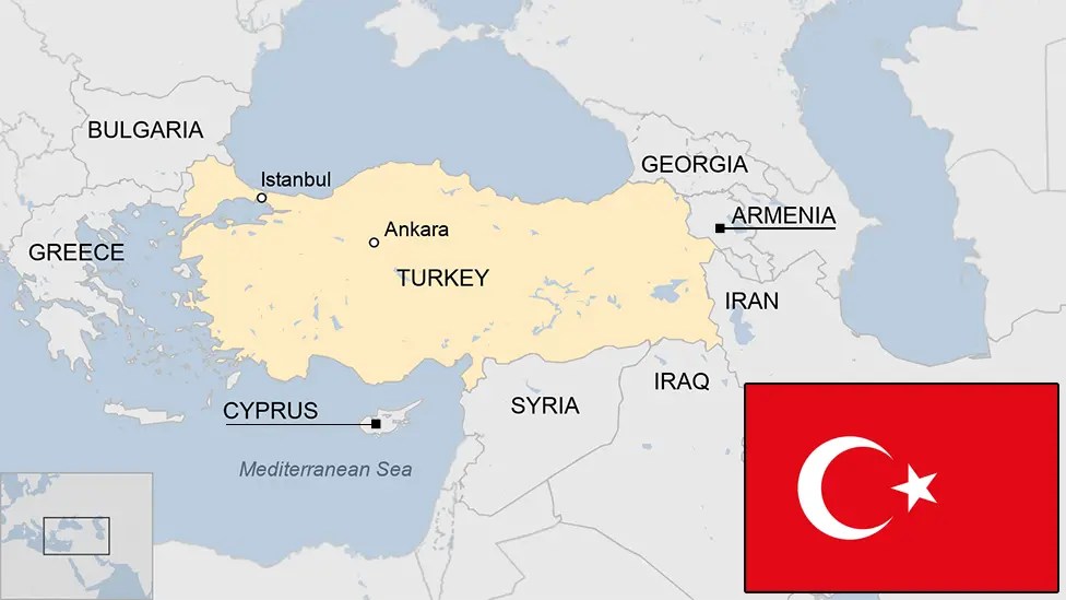
Lastly, in regard to the geopolitical state of the nation, and how this could influence the returns of this trade. Turkey sits at precious position both geographically and politically, as it is positioned at a sensitive crossroad between Europe and the Middle East. Risk-off events could spell sharp USD appreciation, against TRY, which could inhibit on returns. This will have to be watched carefully as we progress in 2026.

Disclaimer: Not financial advice
The Changing Age Demographic of Investing

The FT reported ‘almost a third of UK investors aged over 55 have never heard of exchange traded funds’, which stands in dichotomy to the proposition that ‘an overwhelming 89% of millennials say ETFs are their investment vehicle of choice’, stated by Bloomberg.

Evidence substantiates that the major contradiction between age demographics is most pronounced between Gen Z, Millennials, Gen X, and Boomers. The latter two older generations prefer Mutual funds as their investment vehicle of choice, and the former two prefer ETFs as the bulk of their investing portfolio. Yahoo Finance advances ‘66% of millennials say they could imagine moving to an ETF-only portfolio, whereas only 15% of Boomers say the same’.

The rationale behind the differing investing ethos’s of different generations is clear. Older generations focus on traditional vehicles, and younger generations are importantly still receptive to traditional vehicles like mutual funds, but are credibly more open to new, innovative, investing avenues – unproven in the long term, especially those built on digital platforms.

Reflecting on why younger generations are more adventurous investors with an appetite for high-risk, high-reward avenues. A potential justification that can be proposed is less to do with digitisation more to do with younger generations engaging in dialogues around building wealth. Especially the strategy in how to grow wealth at a compound rate, Gen Z purports that wage-based saving is futile in comparison. As of January 2026, the best instant access saver accounts range from 4.5% AER for Chase. Other banks, such as Lloyds, with their Club Lloyds Saver have variable rates 0.95%-1.20% AER, and HSBC with Online bonus saver, with a standard rate on all balances at 1.15% AER. This is dwarfed by the one of the most popular ETFs, such as the S&P 500 (SPY), that achieved 18% total return last year in 2025, and 25% in 2024, backed by Goldman Sachs.

Yet still, the SPY is a relatively low-risk ETF. If more concentrated ETFs are invested in, with sector or thematic focuses, results delivered can be even more lucrative, but evidently come with more risk appetite. The most profitable ETF in 2025 was the iShares MSCI Global Silver and Metals ETF (SLVP) which recorded a 212% gained, and in addition SILJ with a 195% gain.

With these figures in mind, the logic does not follow on why a wealth-building driven investor would choose a regular savings account over an ETF. This raises the contention, why Gen X and Boomers have a stubbornness for ETFs. A potential reason for this friction may be less doubt-fuelled, and more motivated by tax exposure concerns. To unwind capital from mutual funds to ETFs, it could trigger Capital Gains Tax. Furthermore, since most Boomers have held mutual funds in brokerage accounts for not just years, but decades, the tax exposure is even more extraneous, and could fall into the long-term capital gains tax rate rate. In the UK, this basic rate increased to 18% this past year, and 24% for a higher rate. If a Boomer were to withdraw capital from a mutual fund, the trade-off for transitioning to ETFs would only be worthwhile if the pay-off of an ETF exceeds the performance of the mutual fund, and the lost capital – combined. For example, £1 million in a which earns an average 10% returns a year, if this is withdrawn and faces a 20% capital gains tax rate. The reaming capital invested into an ETF left could be £800,000, the returns of the ETF would have to essentially be greater than 30%, to make this strategy worthwhile.

Even if Boomers were to go ahead with this strategy, or if capital gains tax were reduced, and ETFs’ average returns kept on exceeding their track record, this raises the question on what happens if everyone simply invested in ETFs. The possibility of this reality may be less flawless than expected. The real-time repercussions could be a lack of price discovery, reduced market efficiency, high mispricing risk. A broken market would then produce its own spell of problems.

Disclaimer: Not financial advice.
2026 FX Forecast: SEK & NOK

SWEDEN (SEK)

An up-and-coming theme in FX markets for 2026 may be the actual outperformance of Scandinavian currencies led by Sweden, with the Swedish krona (SEK) set to compete against the euro and the dollar. This is building on significant gains already established from 2025, where SEK was one of the best-performing G10 currencies in late 2025.

This proposition can be backed by analysts from Bank of America who have forecasted for SEK to surge further ahead, with the end-of-year 2026 forecast to be EUR/SEK 10.50 and USD/SEK 8.81. MUFG further purports USD/SEK to be 8.38 by Q4 2026, with its spot close on December 31^st at 9.19.

Breaking down what these exchange rates mean. 1 euro will cost 10.50 Swedish kroner. If the EUR/SEK goes down, from 10.50 to 10.20, this means the krona is becoming stronger. If the exchange rate goes up, from 1 euro to 10.50 to 10.70, it means the krona is becoming weaker. To put into comparison, why 10.50 is considered a strong position, is that previously the exchange rate in January 2025, was 11.54.

Drivers of SEK growth can be pinned down to three main reasons. Foremost, the fiscal picture of the nation, trade and defence spending, and thirdly monetary policy differentials.

The fiscal picture refers to a government’s finances, giving a snapshot of income, spending, debt, and financial sustainability, and also whether a government is running a surplus or deficit, it in essence maps out the picture of public finances. Norway’s fiscal state has been exceptionally strong over the past decade. This is due to a combination of a low debt-to-GDP ratio, which has averaged 33-34%, much lower than the Eurozone goal of 60%. In contrast Italy’s debt-to-GDP ratio is 137%, the UK’s 95%, and the USs 122%. Norway has a stable budget account, its deficit-to-GDP ratio was recorded as 1.7% at the end of the previous year, in comparison the US’s was sitting around 6% for 2025, the UK’s 3.9%. On top of this, Sweden has had controlled government spending, anchored on its framework set out following its 1991-1993 economic crisis.

Trade and Defence spending is a second primary driver. The country aims for 3.5% of GDP to be made up of boosted defence spending by the end of 2026, in tandem with the nation having joined NATO in 2024. This is backed by its already competitive defence and industrial exporters like Saab, BAE Systems – Bofors AB, and Boghammar Marin. This is evermore bolstered by Germany’s and Sweden’s new bilateral defence partnership, the MofU (memorandum of understanding) signed in late 2025. This framework signifies that the two countries have a partnership in areas covering energy and defence.

With respect to the latter assertion on monetary policy differential’s, FX markets don’t necessarily respond if rates are high; on a futile level they respond to what the rates are in comparison to elsewhere. The Riksbank, the oldest central bank in the world, has a crucial rates relationship with the ECB. The ECB has been dovish over the past few years, conducting a rate cutting cycle, which began in June 2024 from its 4.0 % peak, up until its current hold at 2.15% in June 2025. The Riksbank has cut rates from 4% to 1.75% in this same time period. This narrowing differential has been quoted here as one of the primary catalysts, as it reduces the incentive for carry trades. For years, investors sought the low-yielding SEK as a route in which to purchase high-yielding assets, which in turn pushed the Swedish Krona down. This avenue has been negated, as it has forced positions in SEK to be unwound, lifting the SEK back up.

A bonus point to this argument on why the SEK has bee particularly strong, may also be supported by the softening of the dollar and the euro, especially amid contentions of ‘de-dollarisation’, bolstering the currency pair.

NORWAY (NOK).

For Norway, the strength of it’s currency is really about oil prices, less so the monetary or fiscal picture. The NOK is contestably one of the cleanest oil-linked currencies across the globe, with an embedded structural relationship. This is unsurprising since the oil and gas sector contributes approximately 20% to the country’s GDP, and its advantageous position servicing 2% of the world’s oil supply, given the nation’s small population and it being a non-OPEC member. Analysts from BofA predict that by the end of 2026 for USD/NOK to be 9.26, in tandem with the EUR/NOK at 11.30, advocating the same bullish forecast, parallel to SEK.

The monetary picture as touched on, is less pressing in this instance, despite the Norges Bank is still expected to deliver 50 basis points rate cuts in 2026. There is an evident disconnect with rates and FX, which has also been observed with the Yen. The fiscal position of the country, Norway has been consistently robust. The nation routinely runs a large budget surplus which was 13.2% of GDP, propped up by substantial oil and gas revenue and the world’s largest sovereign wealth fund – GPFG.

It is possible the NOK could deliver a twin act with SEK, both outperforming the dollar and euro in 2026. This outcome could come to fruition if Norway makes an ardent effort towards projects related to carbon capture and Storage and low-carbon hydrogen production. These efforts could in turn make Norway’s oil and gas exports more attractive options, pushing the sector further along, especially in a carbon-constrained market.

The only caveat is the potential drag from European pessimism in late 2026 that could come forth, dragging USD/SEK. Nonetheless, any dips in SEK with the euro or the dollar, analysts have advocated that this may serve as a buying opportunity.
Analysing FX Candlesticks
An FX chart is a visual tool to show a currency pair’s past price movements. The map of its movements can be used to predict its future changes, in which to enact speculation, hedging, or arbitrage.

Candlestick charts originated as a measurement tool in Japan in the 18^th century to anticipate the price of rice. Charles Dow (co-founder of Dow Jones and Company) brought them to the attention of the Western Hemisphere, and were then popularised by a trader, Steven Nison, in his book ‘Japanese Candlestick Charting Techniques’ published in 1991.

FX charts can be in the form of line charts, bar charts, or candlestick charts. The most widely used is candlestick charts, especially on an institutional level.

Below shows a typical candlestick chart for the major pair GBP/USD.

The horizontal bars are each a ‘candle’ which represents a time duration, usually a day, but can be adjusted to be a week or a month. The four main features are the open price, the high price, the low price, and the close price. A candlestick with a longer time frame, like a week or a month can portray more reliable trends, a shorter time frame, such as an hour can show more detailed movements, but more movements can equal more noise.

Open price – the first trade during the specified period. (i.e. the first trade of the day).

High price – the highest traded price during the specified period.

Low price – the lowest trade during the specified period.

Close price – the last trade during the specified period.

The image below illustrates this. The colour of the candlestick is an important factor.

A green candlestick reflects a bullish market, as the closing price was higher than the opening price. This suggests buyers have control.

A red candlestick reflects a bearish market, that the closing price was lower than the opening price. This suggests sellers have control.

The shape of the candlesticks can give indicators about what’s to come next, as they can reflect market sentiment. A few key themes portrayed from the following description of candlesticks and their patterns is the importance of a bearish or a bullish signal, and whether it is a sellers and a buyer’s market.

These include:
1. Doji (gravestone, long-legged, and dragonfly)
A Doji (denotes its name from its Japanese translation meaning ‘the same thing’) occurs when the opening and closing prices are almost identical, with a short vertical body, and long wicks. A Doji can indicate that the preceding change can go either way, it exemplifies indecision within the market.
1. Gravestone Doji: This upside-down T ‘gravestone’ shape can signal a potential end of an upward trend, and an incipient downward movement in price action may be forthcoming, i.e., bearish reversal. It can depict traders exiting long positions and/or entering short positions.
2. Long-legged: An equal plus + shape Doji, out of these three Doji candlesticks is the most indecisive signal, the closing price and opening price are identical, signalling the market is conflicted, traders may wait for the next candlestick to act.
3. Dragonfly: This cross-shaped Doji is the opposite of the gravestone Doji and its signal. Again, similar to the latter two examples, both closing and opening prices are almost identical, an incipient upward movement could ensue – a bullish reversal signal.
2. Wide-ranging Candlestick

A wide-ranging bar looks like a long vertical bar, usually 2-3 times the length of any surrounding candlesticks. As depicted below it is easily identifiable, disrupting a pattern. This bar illustrates the open and close price had a substantial difference. A wide-ranging bar in the upward direction, is a strong market indicator, of upward movement. (below). A wide-ranging bar in the downwards direction is strong downward market momentum.

3. Hanging Man & Hammer.

A hammer candlestick and hanging candlestick are essentially the same candlestick in shape, whereby there is a long lower wick, a small body near the top, and little to no upper wick. What determines whether a candlestick falls into each category here is dependent on the surrounding candlesticks.
1. The hanging man is indicative of a bullish reversal. It tells a story that even though during the time period, such as over the course of a day, that even though market prices open high, but prices initially dropped much lower. Ultimately, buyers stepped in enough to reserve this decline, and sustained this through the end of the day. Indicating buyers are in control.
2. Hammers are still identical in shape but can be a bearish reversal of they can be a consequence following a continued downward trend. Hammers are a reliable dictator after a prolonged duration of downward movement, insinuating market sentiment is improving. Under the same precedent as hanging man, buyers are still in control.
4. Inverted hammer and Shooting Star:

This category is the reverse of the previous, where there is a small lower wick, a small body near the bottom, and a large upper wick. Repeatedly, the shape is the same for inverted hammer and shooting star, but what determines if it is one over the other, is relative to the surrounding situation, likewise, to hanging man and hammer, but upside down.
1. The inverted hammer would typically appear when prices have been declining, and a bearish reversal signal may proceed. The long top wick represents a narrative that buyers have been trying to push the price up, but sellers are creating some resistance towards the latter half of the time period or trading day, sellers are therefore in control.
2. A shooting star would usually occur after prices have been increasing, and a bullish reversal could ensue. This shows buyers have been pushing up prices during the time period, but sellers remain in control and pushing down the prices close to what they opened with up until the close.
5. Evening star and Morning star:

This candlestick is a small-bodied, with short wicks at either end, which are usually equal. They show traders are pausing, with little difference between the time durations’ high and low, plus compared to the open and close. The candlesticks importantly appear above or below a previous wide-ranging candlestick, and subsequent wide-ranging candlestick followed, with no overlap over the bodies.
1. An Evening star candlestick, can signal a reliable signal for a bearish reversal, appearing after a peak of uptrends, and can illustrate a moment of pause, where traders do not know if the upward will continue, it is neither a buyer nor a seller’s market for a moment. The following candlestick wicks may be longer, even if the body is still wide-ranging, this portrays a glimpse that sellers are starting to take over and could push down the trend.
2. A Morning star alternatively follows a downward trend, where the previous wide-ranging candlestick has little to no wick, the short body and short wicks repeatedly depict a pause. It is then proceeded by a minute maintenance of the upward trend, but buyers are gaining the slight upper hand and could push up the trend.
Triangles, Flags and Wedges:

The discussion on candlesticks is based on the premise that the time period for each candle is single trading day. When these daily candlesticks are plotted across weeks or months, other patterns can then be discovered from the shapes these candlesticks create. constituting triangles, wedges and flags, which are further indicative tools in which to analyse past movements over a larger time scale and predict future movements further ahead beyond a day.
1. Triangles (ascending, descending and symmetrical):
1. An ascending triangle is a breakout pattern, which is created when a price breaches the straight horizontal upper trendline; this signals a bullish signal. For a pattern to constitute as an ascending triangle, the upper trendline has to be horizontal, which is the resistance line, in which forms a break line – essentially a glass ceiling which has to be broken. This suggests a dominance of higher highs over lower lows. Buyers are dictating this movement, breaking the resistance glass ceiling potentially due to a lack of patience at the current price.
2. A descending triangle is the same situation, alliteratively there are more lower lows over high highs, creating a downward triangle. Sellers are more in control of the market, there is also the glass ceiling called the resistance level, which is pushing down the price. The glass floor, which is the support price holding up the price to a certain level, would be breached by impatient selling off at higher intensity, since it’s a seller’s market.
3. Symmetrical triangle is the third option whereby sellers and buyers are at equal odds with one another. There are equal, high highs and low lows. The consequential peaks and troughs, which are the resistance and support price collide to a middle converging point, creating a pause for the next direction. The precipitating reaction could go either way. Which way the trend breaches the resistance line, whether it is the glass ceiling or glass floor, is a slight predictor for the incumbent reaction.
Understanding Trading Concepts: Option Greeks

What are Options?

Options are a type of financial instrument called a derivative. They derive their value from an underlying asset, such as stocks (e.g. a single stock such as TSLA – Tesla), a stock market index (e.g. NDX, the NASDAQ-100), or exchange-traded fund (SPY – S&P 500 ETF).

An option is crucially a contract; a buyer pays a premium (essentially an up-front fee) to purchase this contract, which gives the buyer a right, but not the obligation to exercise the option. The buyer is not forced in the future to sell or buy an option up until the specified expiration date, as it’s not an obligation. Much like car insurance, where you pay an upfront premium for the future right to exercise a payout if needed, but you may never use this ability to claim outright.

A call option allows the buyer the right to exercise and buy the asset at its strike price up until the contract finishes. A put option stands in dichotomy, with the difference being the right to sell, instead of buy. Call buyers benefit from rising prices; put buyers benefit from falling prices.

Much like a car insurance contract, an options contract loses intrinsic value up until the end of the expiration date, as the buyer of an insurance, the payoff of investing in the insurance has not been utilised. This can be seen as time decay; this decay compounds and speeds up in the very few weeks right before the end.

A basic definition of options allows for understanding how option Greeks work. The Greeks are ways of understanding how an options price is sensitive to changes in different market conditions, and how they affect an options position (i.e. ITM, ATM, OTM). The Greeks are essentially like dashboard warning lights, if a dashboard light comes on, it is less reflective of the symbol seen, and wholly reflective of the underlying change, in this case, a car engine, that would be the option in this example.

The Five Main Greek Options: Delta, Gamma, Theta, Vega, and Rho.

1.Delta Δ – Directional Risk

Delta is the most commonly known Greek option, and measures how much an option’s price changes for a $1 move in the underlying asset. Delta acts as a directional indicator and probability estimate, ranging from -1 to +1, and looks different for a put option and a call option.

Delta matters as a measurement tool, as it indicates directional exposure and can be used for delta hedging. Moreover, delta can approximate the probability of an option expiring ITM.

Call option: Delta range is from 0 to +1.

Put option: Delta ranges from 0 to -1.

For example, a call option with a delta of 0.60, if the stock rises $1.

2. Gamma (Γ) – Delta’s Sensitivity

In trading, gamma is connected to the first Greek option delta, and measures the rate at which an option’s delta changes as the underlying asset moves $1, i.e. indicates how quickly delta will shift. Think of gamma as the delta of the delta.

A high gamma measure indicates that delta could change dramatically with even a small price change. Gamma is highest for ATM, and correspondingly decreases for ITM, and then is at its lowest for OTM. Gamma is used to assess the risk of delta changing.

A high gamma = delta is changing dramatically, with small price moves, and ITM.

A medium gamma = mid-level movement, but more than low gamma, signalling stability, and ATM.

A low gamma = delta is changing slowly, indicating more stability, and less risk from rapid price swings, and OTM.

In other words, delta tells speed, gamma measures relative acceleration.

3. Theta Θ – time decay

Theta is the Greek that measures an option’s sensitivity to the passage of time, holding all else constant. All else constant means any other changes, such as volatility and interest rates, remain static.

In effect, theta represents the rate at which time decay has on the value of an option.

Theta is worked out by dividing the option value by the time (days or years).

Negative theta infers that the option loses value over time; this is the case for most vanilla options, along with both call and put options.

A positive theta means the option’s value augments upwards over time, this can happen for certain exotic structures and/or are in ITM puts.

The maximum level of time decay happens for ATM options. Theta magnitude is small when an option is deep in ITM and deep OTM. Theta is not constant; it increases in magnitude as expiration nears.

Theta is more negative for options at OTM and ITM, as these situations infer high volatility and a higher option premium. Accordingly, it has been exhibited that Theta is not constant; it increases in magnitude as expiration approaches. A small daily theta pertains to a long-dated options, and a large daily theta is related to short dated options.

4. Vega $ν$ – Volatility

Vega is the amount an options price will change, its sensitivity, to a 1% change in the underlying assets’ implied volatility, holding all factors constant.

Vega is calculated by dividing the option value by the volatility of the underlying asset.

High Vega = occurs when options are ATM and have a long time till expiration, this can be due to there being more time given for price fluctuations, which produces uncertainty. High Vega infers an option has the most extrinsic value, and therefore the most sensitive to changes in implied volatility, reflecting market uncertainty. Most long call and long put options have a positive Vega.

Low Vega = Vega decreases as options get closer to expiring or move further into ITM or OTM. Most short options have negative Vega.

Vega is an important indicator as it represents the level of uncertainty and is an important tool to capitalise on in volatile markets. This is due to Vega being able to capture changes in market sentiment, even when the underlying asset’s price remains stable.

5. Rho ρ – Interest rate

Rho is arguably the least used and least important of the Greek options. It is a measure of how the price of an option’s price changes in response to changes with a 1% change in the risk-free interest rate (the interest rate paid on US treasury bills. Rho is typically expressed as a dollar amount. Interest rates have an impact on an option’s value, as they impact the cost of carrying the position over time.

Rho reflects the sensitivity of calls and puts to rate changes. Calls typically gain in value as rates rise, while puts often lose value. Rho is less important.

High Rho = Options with a longer time to expiration have a higher rho, and accordingly are more sensitive to interest rate changes. Call options and long options generally have a positive rho.

Low Rho = Rho is negative for long puts and short calls. This is because higher interest rates decrease put premiums. High interest rate environments mean a long put is less favourable.
The Three Ways of Looking at Derivatives
Derivatives are financial contracts where the value is derived from an underlying asset, such as a stock, bond, interest rate, commodity, or index. Derivatives are used to manage risk through hedging, speculate on the underlying price movements, or trade with leverage, without having to buy the asset itself. Derivatives come in the form of options and futures. Other forms of a derivative can also exist in the form of spread betting or contract for difference (CFD) trading, which speculate on the price movements of a derivative; these latter two types still constitute as derivatives, as they track the price of an underlying asset.

Derivatives can be seen from 3 different lenses.
1. Rights vs. Obligated based:
Rights-based derivatives

Rights-based deirvatives give the holder the right but not the obligation to buy or sell an asset; options fall into this category.

A key feature of rights-based derivatives is that the holder, once they pay a premium and possess the contract, controls the right on whether to exercise. The rights lay in the holder’s control. The seller (also called the writer) who essentially sold the contract, has an obligation to fulfil the contract at the holder’s request. The pay-off of a rights-based derivative is asymmetric; moreover, the Greeks apply here.

Hedgers would use rights-based derivatives, as this type of derivative can be used to protect against adverse price movements, keep upside potential, and pay a premium as a form of insurance. A hedger would use a rights-based derivative to reduce risk, not necessarily as a profit-maximising tool.

Alternatively, a speculator would see a rights-based derivative as a bet on direction and volatility, limiting downside risk and offering high leverage. A trader would purchase a call option expecting a sustained upward trend in the stock price.

Obligation-based derivatives

Obligation based on the other hand, is where the buyer and seller both have an obligation to conduct a transaction at a future date. This can be forwards, futures, or swaps. At maturity, both parties have no choice but to fulfil the terms of the contract. An obligation-based derivative typically has no upfront premium, except for margin (this collateral, however, is not necessarily a cost).

An obligation-based derivative pay-off looks slightly different, as it has a symmetric payoff; there is unlimited profit and loss potential. One party’s gain is one party’s loss. However, the Greeks do not apply here.

In other words, what could be seen as what determines whether a derivative is considered rights or obligation based is based on the condition of the holder (the buyer) of the contract, as the deciding factor.

Hedgers can use obligation-based derivatives to lock in prices to ensure certainty, eliminating both upside and downside risk. For example, a client who is an airline, may use fuel futures to lock in fuel costs to avoid future price uncertainty.

Alternatively, a speculator would use an obligation-based derivative to make a strong directional position, ensuring no premium risk, with a high risk, high reward. For example, a trader purchasing an index future may be under the guise of the market to rising.

2. Linear vs. Non-Linear

Derivatives categorised under this lens are distinguished via their payoff structure. Payoff is the profit or loss of a derivative from the contract.

Linear Derivatives

Linear derivatives have a pay-off structure that changes proportionally, i.e., one-to-one with the price of the underlying asset. A 1-unit change in the underlying asset causes a 1-unit change in the derivative value. Therefore, payoff is symmetric; equal upside and equal downside, but the gains and losses are unlimited.

Linear derivatives are forwards, futures, and swaps, they have little convexity; the Greeks do not apply.

Linear derivatives are used by hedgers to lock in prices or rates and remove uncertainty from future cash flows. Speculators see linear derivatives as a way to gain high leverage, and arbitrageurs use them to exploit price mispricing, ensuring price alignment between spot and derivative markets, which in turn can accumulate low-risk profits.

Those aiming for arbitrage can use linear derivatives to exploit mismatches between spot and derivative markets.

Non-Linear Derivatives

Conversely, non-linear derivatives have a payoff that is non-proportional to the underlying asset price. These refer to instruments which involve optionality and volatility, e.g. a call option.

Non-linear derivatives provide an asymmetric risk-return; losses are often limited for the buyer. Common examples include call and put options, plus exotic options (barrier, digital, Asian)

This means that the asset’s price, and its sensitivity (the delta) changes with price, time, and volatility. The pay-off when graphed is convex or concave, rather than a straight line seen for linear derivatives.

Non-linear derivatives are used by hedgers to obtain downside protection whilst retaining upside potential, by speculators to benefit from leverage and volatility-based strategies, and by institutions to create bespoke structured products.

3. Exchange-traded vs. Over-The-Counter:

The third, and most popular, lens on which to see derivatives and how to separate them, is based on the location derivatives are traded, i.e., on or off a market. The derivatives market is not a single physical place, but rather a point where buyers and sellers meet to partake in an exchange. This can be on a listed exchange, such as the CME (Chicago Mercantile Exchange) or ICE (International Exchange).

Exchange Traded Derivatives (ETDs)

ETDs are standardised derivative contracts traded on organised exchanges, such as those like the CME or ICE. They are cleared through a central clearing house in order to lower default risk. Since ETDs are standardised financial contracts, they have set out details such as the size, maturity, and strike price. For example, ETDs can be futures, commodity derivatives, or vanilla options.

The main benefit of ETDs over OTC derivatives is the high-level standardisation and regulation, this consequently results in low counterparty risk, this results in the products offering a higher level of transparency and liquidity. For corporations these can be beneficial for more tailored risk management. For institutions when increased complex and large transactions are conducted, ETDs are suitable.

Over-the-Counter Derivatives (OTC Derivatives)

Opposingly, OTC derivatives happen off an exchange. They essentially happen on a private market, as these are privately negotiated bilateral agreements, traded directly between two parties. There is no presence of a central exchange. This results in high counterparty risk and less transparency. The customised nature results in higher flexibility, meaning exact hedging is possible.

OTC derivatives offer less liquidity, with only light regulation. These derivatives are still overseen by collateral regulation. Examples of OTC derivatives include forwards, swaps, and exotic options.
Company Profile: What’s Next for Wells Fargo?

14th January, 2026

Well Fargo’s path to stability, following the annulment of their asset cap, is not looking so straightforward. This is in lieu of their Q4 financial data being published on January 14^th. Where the bank reported it missed its profit estimates, with shares subsiding 4.8% to a share price of $89.

It’s been only seven months since their infamously punitive, $1.95 trillion asset cap was lifted. Since this restriction was imposed in 2018, it has seen its investment banking revenue stagnant below $1billion year on year since. Relative to its counterparties Goldman and JPMorgan, whom at their peak in 2021-2022 achieved up to $3.5 billion revenue.

Under Charlie Scharf’s direction, the bank sees its strategy in catching up, a deviation from what caused their predicament in the first place. Their 173-year-old history was built on an all-American consumer ethos that came first, and stood as a pillar of its branding. This arguably metamorphosized into what became their Achilles heel. Their cross-selling scandal involved the bank opening millions of unauthorised bank accounts and credit cards for customers. Forging fake records and signatures, damaging customers credit scores and incurring fees on accounts. This indubitably damaged their reputation, and heavily their balance sheet following the financial sanctions.

Potentially this divergence is an attempt to separate itself from this consumer banking identity, instead focusing on solidifying itself as a refined investment bank, potentially on a par with Morgan Stanley who do offer commercial banking, but not at a foremast of its business model. Remnants of this effort are starting to be picked up. At the end of December 2025, six months since the revocation, Fargo has had a transaction resurgence, and has managed to ascend the LSEG M&A rankings from 17^th place to 9^th.

Wells Fargo’s aggresive transactions tactic is observed with Fargo being one of the primary financing lenders to Netflix for the incipient Warner’s Brothers acquisition. Fargo extending a $59 billion bridge loan, is a pertinent distinction of Fargo’s uncompromising method, as it is one of the largest ever bridging loans observed from any company, to finance an acquisition. This $59 billion dwarfs BNP’s $20.7 billion contribution, in addition to HSBC’s $9 billion addition.

Scharf has publicly announced he aims for Wells Fargo to be considered a top 5 investment bank globally. Scarf it appears is attempting to achieve this by changing the shape of its workforce. 25 Managing Directors are intended to be hired in 2026, with a focus on healthcare, technology, and industrials. Nonetheless, the people power behind transactions and the brand– analysts and associates – are anticipated to see a cut in numbers, in attempt to drive efficiency with increased AI refinement. This is a continuation stemming from the beginning of Scarf’s tenure in 2019, which has seen the workforce shrink from 275,000 in 2019 to 210,000 to 2025.

In terms of whether Wells Fargo can achieve this vision, the strategy of focusing on revenue driving sources seems to be the best outlook, after lost trust with consumers. Rebuilding consumer reputation has a longer trajectory and timeline. In comparison, client reputation can be easier rebuilt by involvement in landmark deals. Deploying MDs in growth sectors, in which to create, and potentially re-define client relationships appears the right approach on which to do this and climb rankings.

The remaining qualm is whether Wells Fargo culture of aggressive targets for staff has been resolved. If the bank can remedy unethical practises and can crucially sustain strong involvement in leading upcoming deals in 2026, including those of the likes of OpenAI, Broadcom, Nvidia, and Microsoft Azure, its future which involves the bank being taken seriously again as a major player, seems favourable.